

How To Draw Qq Plot In Excel
Histogram
A histogram can be used to determine whether data is normally distributed. This test consists of looking at the histogram and discerning whether it approximates the bell curve shape of a normal distribution.
Example 1: Determine whether the data in column B of Figure 1 are normally distributed using a histogram.

Figure 1 – Testing for normality using a histogram
The sample contains 20 data elements. To make sure that the intervals in the histogram are equal and consistent, we first standardize the data points (in column C) as described in Expectation. E.g. the formula in cell C4 is =STANDARDIZE(B4,$B$24,$B$25). Choosing bins from -2 to 2 standard deviations, we create a histogram as described in Histograms.
As you can see from Figure 1, the histogram doesn't look particularly normal in shape. Caution should be exercised when using a histogram to test for normality since the choice of bin sizes may have a dramatic effect on the result. See Histograms for how to choose the correct bin size.
QQ Plot
A PP plot (point-point plot) is simply a scatter plot comparing two samples of the same size. The more similar the underlying distributions, the more closely the scatter points will conform to a line with slope 1. If the data are standardized then the scatter points would be close to the line y = x.
We can also use a PP plot to compare a data set with a distribution. If the distribution has cdf F(x) and the data set has elements x 1, …, xn in ascending order, then the PP plot is the scatter diagram of the set {F(x 1), …, F(xn )} versus the set {1/2n, 3/2n, …, 1−1/2n}. Here the second set is an attempt to divide the interval between 0 and n into n evenly spaced intervals (except for the first and last elements which are half the length).
A QQ plot (quantile-quantile plot) is also used to compare a data set with a distribution, and consists of a scatter plot of the data set {x 1, …, xn } in ascending order with the values {F -1(1/2n), F -1(3/2n), …, F -1(1−1/2n)}. Here the ith value F -1(i/n−1/2n) is the inverse of the cdf at i/n−1/2n (these are the quantiles).
As for PP plots, if the points on the scatter plot align with the diagonal line y = x then the data set conforms with the distribution.
When using a QQ plot to see whether a data set is normally distributed, you create a scatter diagram between range R1 consisting of the elements x 1, …, xn in ascending order and R2 consisting of the values NORM.INV(1/2n, x̄ , s), …, NORM.INV(1−1/2n, x̄ , s), where x̄ = AVERAGE(R1) and s = STDEV.S(R1).
Alternatively, you can create a scatter diagram between range R1 consisting of the standardized elements z 1, …, z n , where each zi = STANDARDIZE(xi , x̄ , s), and range R2 consisting of the values NORM.S.INV(1/2n), …, NORM.S.INV(1−1/2n).
A QQ plot is used much more often than a PP plot. PP plots tend to magnify deviations from the distribution in the center, QQ plots tend to magnify deviation in the tails.
Example 2: Using a QQ plot determine whether the data set with 8 elements {-5.2, -3.9, -2.1, 0.2, 1.1, 2.7, 4.9, 5.3} is normally distributed.
The mean of this data set is .375 and the standard deviation is 3.89. If the data set is normally distributed then for any value x, the cumulative distribution at x would be given by
F(x) = NORM.DIST(x, .375, 3.89, TRUE)
We now split the interval (-∞, ∞) into 8 sub-intervals (-∞, x 1 ), (x 1, x 2), …, (x 7, x 8), (x 8, ∞) such that the area under the standard normal curve for the 2nd through 7th intervals are equal and the area under the curve of the first and last intervals are half the size of the middle intervals. This is equivalent to finding points z 1 , z 3 , z 5 , z 7 , z 9 , z 11 , z 13 and z 15 such that zi = NORM.S.INV(i/16). Thus xi = z 2 i- 1 and if the original data are normally distributed then
F(xi ) = NORM.S.INV((2i–1)/16).
We summarize this approach in Figure 2, where we have also standardized the original data so that it is easier to compare the standardized data with the standard normal approximation for each data point (under the assumption that the original data are normally distributed). Finally, we have included a scatter diagram (the QQ plot) of the data vs. the standardized normal data.
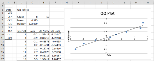
Figure 2 – Using a QQ plot to test for normality
Cells E5. D6 and D7 contain the formulas =2*COUNT(A4:A11), AVERAGE(A4:A11) and STDEV.S(A4:A11). The range D10:D17 contains the data in sorted order, e.g. by using the formula =QSORT(A3:A11). Cell E10 contains the formula =NORM.S.INV(C10/E5) and cell F10 contains the formula =STANDARDIZE(D4,D$6,D$7), and similarly for the other cells in columns E and F.
We then create a scatter chart from the data in range E10:F17 (as described in Excel Charts) and add a linear trend line (as described in Scatter Plots).
We can see that the data pretty well fits with the trend line, which is a good indicator that the original data is roughly normal. In fact, if the original data is normally distributed, then when the standardized data is plotted against the standard normal values the trend line should be the diagonal line through the origin y = x.
QQ Plot Data Analysis Tool
Real Statistics Data Analysis Tool: The Descriptive Statistics and Normality data analysis tool contained in the Real Statistics Resource Pack allows you to create QQ plots automatically. We illustrate this capability in the following example.
Example 3: Determine whether the data in Example 1 is normal by using a QQ plot. The data is repeated in range A3:A23 of Figure 4.
To run the analysis, press Ctrl-m and select the Descriptive Statistics and Normality option (from the Desc tab when using the multipage user interface). Fill in the dialog box that appears as shown in Figure 3, choosing the QQ Plot option, and press the OK button.

Figure 3 – QQ Plot dialog box
When you click on the OK button, the output shown in Figure 4 is displayed.

Figure 4 – QQ plot for data in Example 1
This time you can see that the data is not particularly normally distributed.
Box Plots
While box plots can't actually be used to test for normality, they can be useful in testing for symmetry, which sometimes is a sufficient substitute for normality.
Example 4: Use a box plot to gain more evidence as to whether the data in Example 1 is symmetric.
To produce the box plot, press Ctrl-m and select the Descriptive Statistics and Normality option. Fill in the dialog box that appears as shown in Figure 3, choosing theBox Plot option instead of (or in addition to) the QQ Plot option, and press the OK button. The output is shown in Figure 5.

As we can see from Figure 5, the data is relatively symmetric, and so although as we saw in Example 1 and 3, the data is probably not normally distributed, it does appear to be relatively symmetric, which is sufficient for some of the tests that we would like to use.
References
Howell, D. C. (2010)Statistical methods for psychology (7th ed.). Wadsworth, Cengage Learning.
https://labs.la.utexas.edu/gilden/files/2016/05/Statistics-Text.pdf
How To Draw Qq Plot In Excel
Source: https://www.real-statistics.com/tests-normality-and-symmetry/graphical-tests-normality-symmetry/
Posted by: brownbefor1967.blogspot.com
0 Response to "How To Draw Qq Plot In Excel"
Post a Comment